Lasso Regression

Lasso regression is a statistical model that combines linear/logistic regression with L1 regularization to perform both variable selection and regularization. The term “Lasso” stands for “Least Absolute Shrinkage and Selection Operator.” This method is particularly useful when dealing with datasets that have many predictors, as it helps to: - Reduce overfitting by penalizing large coefficients - Perform automatic feature selection by shrinking some coefficients to exactly zero - Handle multicollinearity by selecting only one variable from a group of highly correlated predictors

In this analysis, we’ll use Lasso regression to predict weapon carrying behavior in schools, demonstrating how this method can help identify the most important predictors while maintaining model interpretability.

Setting Up the Environment

First, we need to load the necessary packages for our analysis. We’ll use tidymodels for modeling, tidyverse for data manipulation, and here for consistent file paths.

library(here)
library(tidymodels)
library(tidyverse)

Loading the Data

We’ll work with pre-processed data sets that have been split into training and test sets, along with cross-validation folds. These files are stored in the processed_data directory.

analysis_data <- readRDS(here("models", "data", "analysis_data.rds"))
analysis_train <- readRDS(here("models", "data", "analysis_train.rds"))
analysis_test <- readRDS(here("models","data", "analysis_test.rds"))
analysis_folds <- readRDS(here("models", "data", "analysis_folds.rds"))

Data Preprocessing

Before fitting our model, we need to preprocess the data. We’ll create a recipe that: - Imputes missing values in categorical variables using the mode - Imputes missing values in numeric variables using the mean - Removes predictors with zero variance - Removes highly correlated predictors (correlation threshold = 0.7) - Creates dummy variables for categorical predictors

weapon_carry_recipe <- 
  recipe(formula = WeaponCarryingSchool ~ ., data = analysis_train) |>
  step_impute_mode(all_nominal_predictors()) |>
  step_impute_mean(all_numeric_predictors()) |>
  step_zv(all_predictors()) |> 
  step_corr(all_numeric_predictors(), threshold = 0.7) %>% 
  step_dummy(all_nominal_predictors())

weapon_carry_recipe

── Recipe ──────────────────────────────────────────────────────────────────────

── Inputs 

Number of variables by role

outcome:    1
predictor: 10

── Operations 

• Mode imputation for: all_nominal_predictors()

• Mean imputation for: all_numeric_predictors()

• Zero variance filter on: all_predictors()

• Correlation filter on: all_numeric_predictors()

• Dummy variables from: all_nominal_predictors()

Let’s apply our recipe to transform the data according to these preprocessing steps.

weapon_carry_recipe %>% 
  prep() %>% 
  bake(new_data = analysis_data) 

# A tibble: 19,595 × 11
   WeaponCarryingSchool AttackedInNeighborhood_X1 Bullying_X1
   <fct>                                    <dbl>       <dbl>
 1 0                                            0           0
 2 0                                            0           1
 3 0                                            0           0
 4 0                                            0           0
 5 0                                            0           0
 6 0                                            1           0
 7 0                                            0           0
 8 0                                            0           0
 9 0                                            0           0
10 0                                            0           0
# ℹ 19,585 more rows
# ℹ 8 more variables: SexualAbuseByOlderPerson_X1 <dbl>,
#   ParentalPhysicalAbuse_X1 <dbl>, ParentSubstanceUse_X1 <dbl>,
#   ParentIncarceration_X1 <dbl>, SchoolConnectedness_X1 <dbl>,
#   ParentalMonitoring_X1 <dbl>, UnfairDisciplineAtSchool_X1 <dbl>,
#   Homelessness_X1 <dbl>

Model Specification

We’ll use a logistic regression model with Lasso regularization. The Lasso (Least Absolute Shrinkage and Selection Operator) helps with feature selection by penalizing the absolute size of coefficients. We set mixture = 1 to specify a pure Lasso model, and we’ll tune the penalty parameter to find the optimal level of regularization.

weapon_carry_spec <-
  logistic_reg(penalty = tune(), 
               mixture = 1) |> 
  set_engine('glmnet')

weapon_carry_spec

Logistic Regression Model Specification (classification)

Main Arguments:
  penalty = tune()
  mixture = 1

Computational engine: glmnet 

Creating the Workflow

We’ll combine our recipe and model specification into a single workflow. This ensures that all preprocessing steps are properly applied during both training and prediction.

weapon_carry_workflow <-
  workflow() |>
  add_recipe(weapon_carry_recipe) |>
  add_model(weapon_carry_spec)

weapon_carry_workflow

══ Workflow ════════════════════════════════════════════════════════════════════
Preprocessor: Recipe
Model: logistic_reg()

── Preprocessor ────────────────────────────────────────────────────────────────
5 Recipe Steps

• step_impute_mode()
• step_impute_mean()
• step_zv()
• step_corr()
• step_dummy()

── Model ───────────────────────────────────────────────────────────────────────
Logistic Regression Model Specification (classification)

Main Arguments:
  penalty = tune()
  mixture = 1

Computational engine: glmnet 

Model Tuning

To find the optimal penalty value, we’ll create a grid of potential values to test. We’ll use 50 different penalty values, evenly spaced on a logarithmic scale.

lambda_grid <- grid_regular(penalty(), levels = 50)
lambda_grid

# A tibble: 50 × 1
    penalty
      <dbl>
 1 1   e-10
 2 1.60e-10
 3 2.56e-10
 4 4.09e-10
 5 6.55e-10
 6 1.05e- 9
 7 1.68e- 9
 8 2.68e- 9
 9 4.29e- 9
10 6.87e- 9
# ℹ 40 more rows

Now, we’ll perform cross-validation to find the best penalty value. This process is time-consuming, so we’ll save the results for future use.

set.seed(2023)

lasso_tune <- 
  tune_grid(
  object = weapon_carry_workflow, 
  resamples = analysis_folds,
  grid = lambda_grid, 
  control = control_resamples(event_level = "second")
)

Let’s examine the performance metrics for different penalty values.

lasso_tune %>% 
  collect_metrics()

# A tibble: 150 × 7
    penalty .metric     .estimator  mean     n std_err .config              
      <dbl> <chr>       <chr>      <dbl> <int>   <dbl> <chr>                
 1 1   e-10 accuracy    binary     0.957     5 0.00158 Preprocessor1_Model01
 2 1   e-10 brier_class binary     0.881     5 0.00160 Preprocessor1_Model01
 3 1   e-10 roc_auc     binary     0.688     5 0.00742 Preprocessor1_Model01
 4 1.60e-10 accuracy    binary     0.957     5 0.00158 Preprocessor1_Model02
 5 1.60e-10 brier_class binary     0.881     5 0.00160 Preprocessor1_Model02
 6 1.60e-10 roc_auc     binary     0.688     5 0.00742 Preprocessor1_Model02
 7 2.56e-10 accuracy    binary     0.957     5 0.00158 Preprocessor1_Model03
 8 2.56e-10 brier_class binary     0.881     5 0.00160 Preprocessor1_Model03
 9 2.56e-10 roc_auc     binary     0.688     5 0.00742 Preprocessor1_Model03
10 4.09e-10 accuracy    binary     0.957     5 0.00158 Preprocessor1_Model04
# ℹ 140 more rows

We can visualize how the model’s performance changes with different penalty values.

autoplot(lasso_tune)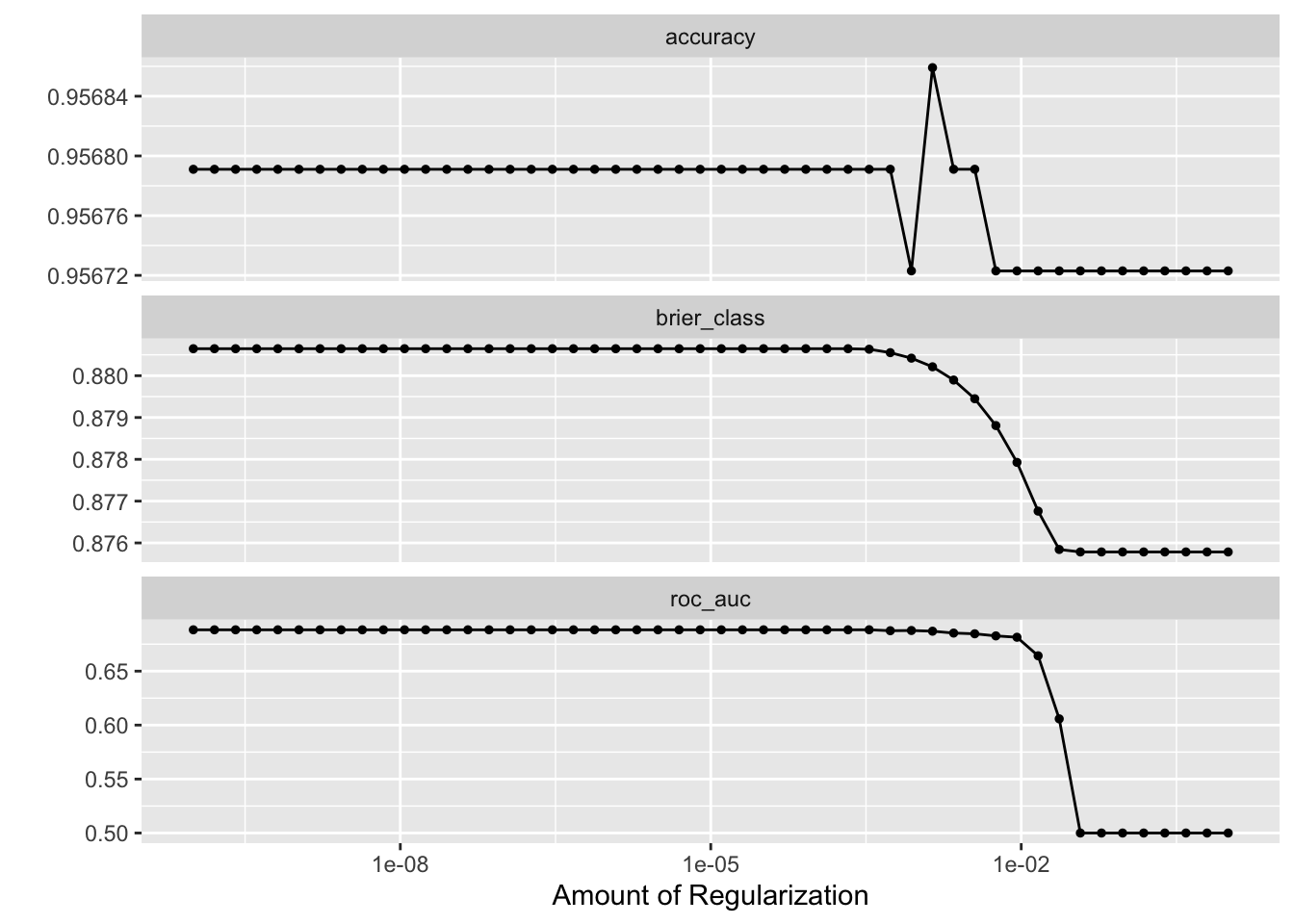

Selecting the Best Model

We’ll select the best model based on the ROC AUC metric, which measures the model’s ability to distinguish between classes.

best <- lasso_tune |> 
  select_best(metric ="roc_auc")

best

# A tibble: 1 × 2
   penalty .config              
     <dbl> <chr>                
1 0.000339 Preprocessor1_Model33

Now we’ll create our final workflow with the best penalty value.

final_wf <- finalize_workflow(weapon_carry_workflow, best)

final_wf

══ Workflow ════════════════════════════════════════════════════════════════════
Preprocessor: Recipe
Model: logistic_reg()

── Preprocessor ────────────────────────────────────────────────────────────────
5 Recipe Steps

• step_impute_mode()
• step_impute_mean()
• step_zv()
• step_corr()
• step_dummy()

── Model ───────────────────────────────────────────────────────────────────────
Logistic Regression Model Specification (classification)

Main Arguments:
  penalty = 0.000339322177189533
  mixture = 1

Computational engine: glmnet 

Fitting the Final Model

We’ll fit our final model on the training data. This process is also time-consuming, so we’ll save the results.

weapon_fit <- 
  fit(final_wf, data = analysis_train)

weapon_fit

Model Evaluation

Let’s examine the model’s predictions on the training data.

weapon_pred <- 
  augment(weapon_fit, analysis_train) |> 
  select(WeaponCarryingSchool, .pred_class, .pred_1, .pred_0)

weapon_pred

# A tibble: 14,696 × 4
   WeaponCarryingSchool .pred_class .pred_1 .pred_0
   <fct>                <fct>         <dbl>   <dbl>
 1 0                    0            0.0368   0.963
 2 0                    0            0.0410   0.959
 3 0                    0            0.0253   0.975
 4 0                    0            0.0325   0.968
 5 0                    0            0.125    0.875
 6 0                    0            0.0368   0.963
 7 0                    0            0.0208   0.979
 8 0                    0            0.0208   0.979
 9 0                    0            0.0458   0.954
10 0                    0            0.0529   0.947
# ℹ 14,686 more rows

We can visualize the model’s performance using an ROC curve.

roc_plot_training <- 
  weapon_pred |> 
  roc_curve(truth = WeaponCarryingSchool, .pred_1, event_level = "second") |> 
  autoplot()

roc_plot_training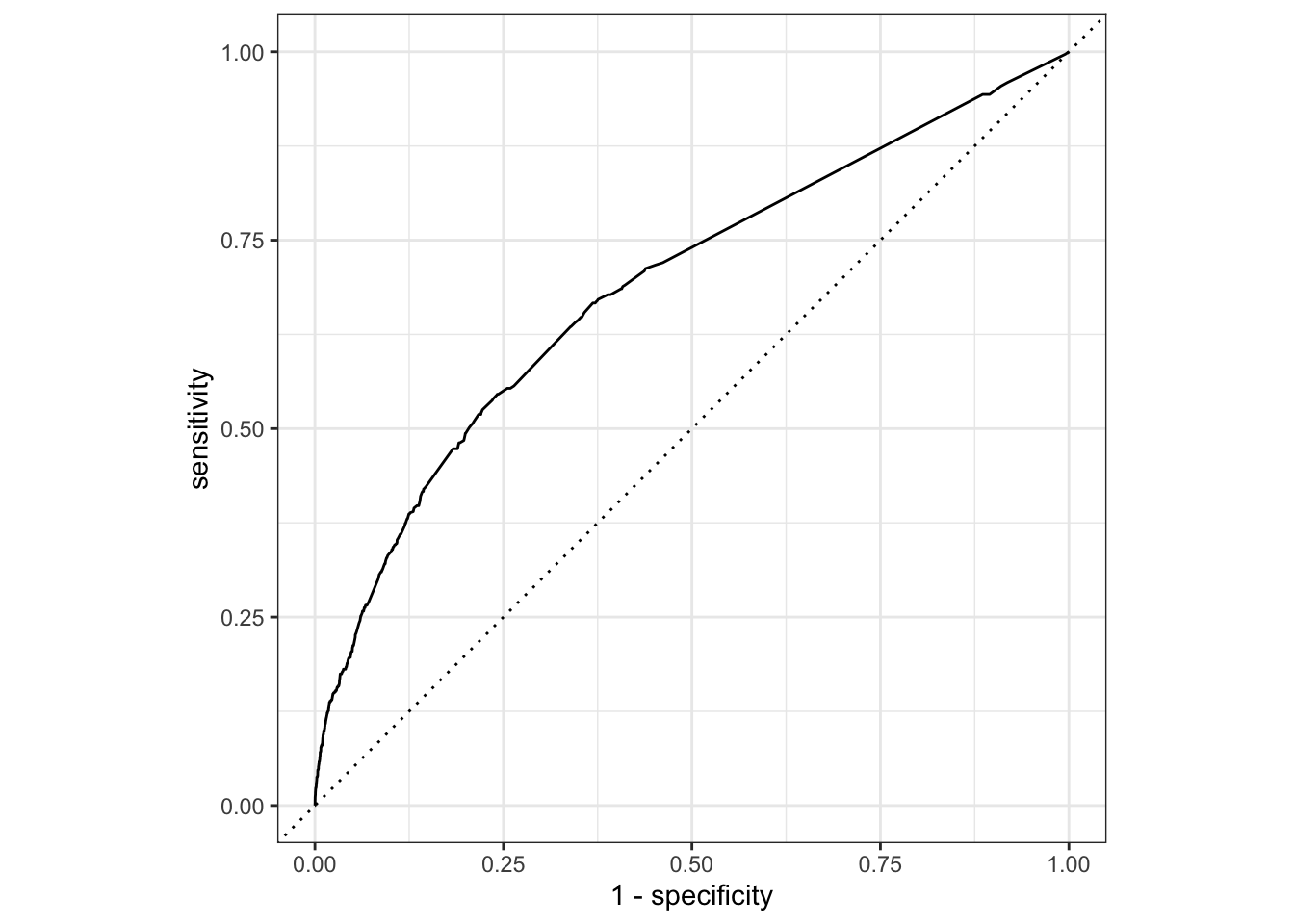 

Let’s look at the model coefficients to understand which predictors are most important.

weapon_fit |> 
  extract_fit_parsnip() |> 
  tidy()

Attaching package: 'Matrix'

The following objects are masked from 'package:tidyr':

    expand, pack, unpack

Loaded glmnet 4.1-8

# A tibble: 11 × 3
   term                        estimate  penalty
   <chr>                          <dbl>    <dbl>
 1 (Intercept)                  -3.29   0.000339
 2 AttackedInNeighborhood_X1     0.739  0.000339
 3 Bullying_X1                   0.472  0.000339
 4 SexualAbuseByOlderPerson_X1   0.455  0.000339
 5 ParentalPhysicalAbuse_X1      0.708  0.000339
 6 ParentSubstanceUse_X1        -0.132  0.000339
 7 ParentIncarceration_X1        0.0271 0.000339
 8 SchoolConnectedness_X1       -0.226  0.000339
 9 ParentalMonitoring_X1         0.584  0.000339
10 UnfairDisciplineAtSchool_X1  -0.229  0.000339
11 Homelessness_X1               1.17   0.000339

Cross-Validation Results

We’ll fit the model on each cross-validation fold to get a more robust estimate of its performance.

weapon_fit_resamples <- 
  fit_resamples(final_wf, resamples = analysis_folds)

weapon_fit_resamples

Let’s examine the cross-validation metrics.

collect_metrics(weapon_fit_resamples)

# A tibble: 3 × 6
  .metric     .estimator   mean     n std_err .config             
  <chr>       <chr>       <dbl> <int>   <dbl> <chr>               
1 accuracy    binary     0.957      5 0.00158 Preprocessor1_Model1
2 brier_class binary     0.0399     5 0.00128 Preprocessor1_Model1
3 roc_auc     binary     0.688      5 0.00737 Preprocessor1_Model1

Variable Importance

Finally, let’s create a variable importance plot to identify the most influential predictors in our model.

library(vip)

Attaching package: 'vip'

The following object is masked from 'package:utils':

    vi

weapon_fit |> 
  extract_fit_engine() |> 
  vip()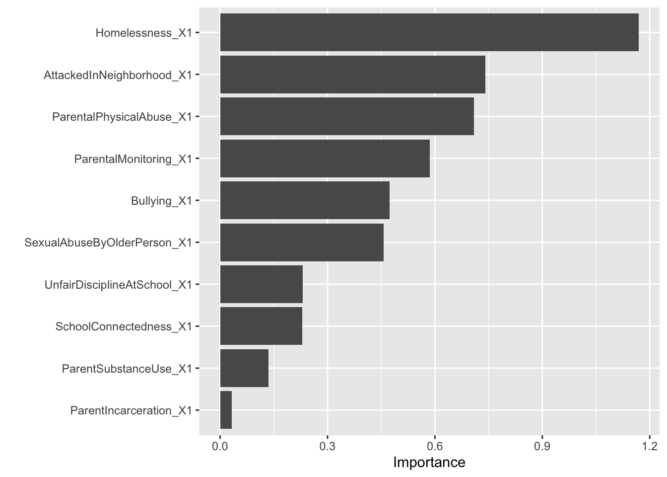 

Results and Interpretation

[Add your interpretation of the results here]